
The reverse DCF is the most useful valuation tool most investors have never run. A forward DCF asks you to forecast the future and hands you a target price built almost entirely on that forecast. A reverse DCF does the opposite: it takes the one number that is not a guess — the price — and solves for the growth the market is already assuming.
Section 1: The Problem
Why the Forward DCF Fails Most Investors
Before the reverse DCF can be understood, the tool it replaces has to be dismantled — the standard forward discounted cash flow, the valuation method every investor is taught and almost no one uses well. A forward DCF asks the analyst to project a company’s cash flows years into the future, choose a growth rate, choose a discount rate, and solve for what the business is worth. The output arrives with the appearance of precision: a single dollar value, carried to two decimal places, that says whether the stock is cheap or dear.
That precision is an illusion, because the answer is almost entirely determined by the growth rate the analyst plugs in — a number nobody can actually know. Change the growth assumption by two percentage points and the “intrinsic value” swings by thirty, forty, fifty percent. The discount rate does the same. The model looks like analysis, but it is really a machine that takes a guess about the future and amplifies it into a target price. The guess is doing all the work, and the model is just dressing it up.
This is why the forward DCF is so easy to fool oneself with. An investor who wants a stock to be cheap can make it cheap: nudge the growth rate up a little, and the model obligingly produces a value above the current price. An investor who is bearish can make the same stock look expensive with an equally small nudge in the other direction. Because the analyst supplies the single most important input, the forward DCF tends to confirm whatever the analyst already believed. Most investors sense this, which is why so many quietly abandon the DCF as an academic exercise that never survives contact with a real decision.
But there is one number in valuation that is not a guess: the current price. The market prints it every second, and that price already contains an embedded forecast — a set of expectations about future growth that, taken together, justify it. Instead of supplying a growth rate and solving for value, an investor can take the price as given and solve for the growth rate the market is already assuming. That single inversion is the reverse DCF, and it turns valuation from a guessing game into a judgment about whether the market’s own expectation is achievable.
The reverse DCF does not ask what a business is worth. It asks what the market already believes — and then lets the investor decide whether that belief is too optimistic, too pessimistic, or about right. It is the single most useful valuation tool available to a long-term investor, and it is the method Quality Equities applies to every business it covers.
Section 2: The Inversion
What a Reverse DCF Actually Is
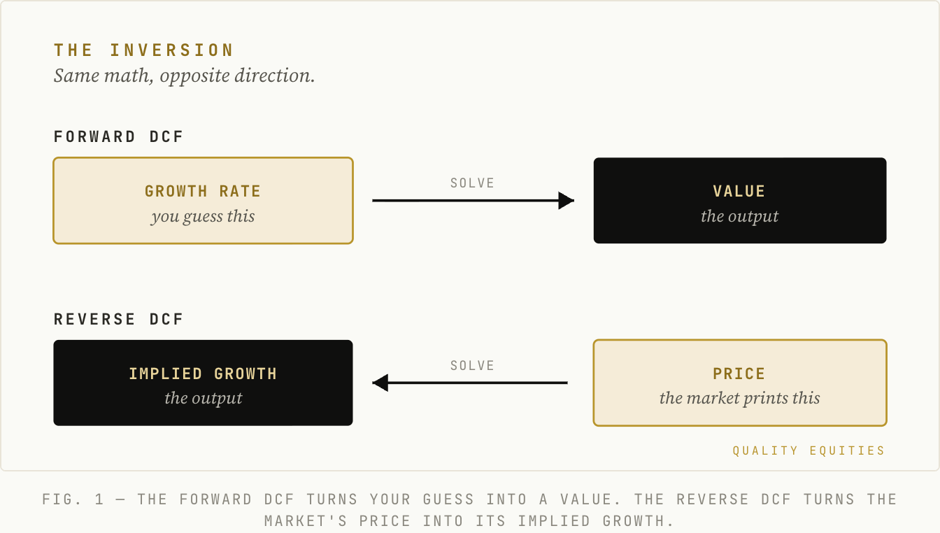
A reverse DCF takes the current stock price as the answer and solves backward for the assumption that produces it — specifically, the rate of growth in owner earnings (or free cash flow) that the market must be expecting in order to justify the price today. A normal DCF runs in one direction: assumptions in, value out. A reverse DCF runs the other way: price in, implied assumption out. It is the same underlying math, executed in reverse. Nothing about the machinery changes; only the unknown does.
The reason the inversion matters so much is that the hardest and least reliable part of any valuation is forecasting growth, and the reverse DCF removes that burden entirely. It does not ask the investor to predict the future. It asks the investor to evaluate a prediction the market has already made. Judging whether a specific growth rate is plausible for a business one understands is a far more tractable task than conjuring that growth rate from a blank page. The reverse DCF converts an impossible forecasting problem into a manageable judgment problem — and judgment, applied to a business inside one’s circle of competence, is where an investor can actually add value.
The mindset this creates has a name: expectations investing, a framework developed by Michael Mauboussin and Alfred Rappaport, who argued that stock prices are best understood as bundles of embedded expectations and that the analyst’s job is to read those expectations rather than to manufacture forecasts. The reverse DCF is the practical engine of that idea. It reframes the entire question of whether a stock is attractive. The investor is no longer asking “will this company grow?” but “will this company grow faster than the market already expects?” A wonderful business can be a poor investment when the market expects even more than it can deliver; a mediocre business can be a fine investment when the market expects almost nothing and it delivers slightly more. The reverse DCF makes those expectations explicit, so the investor is betting on the gap between reality and expectation rather than on the business in isolation.
Section 3: The Method
How to Run a Reverse DCF, Step by Step
A reverse DCF uses the same machinery as a forward DCF — projected cash flows, a discount rate, a terminal value — but instead of solving for value, it holds the value fixed at the current market capitalization and solves for the growth rate that makes the model output equal to that market cap. A motivated reader can replicate the entire exercise in a spreadsheet. The steps are as follows.
Step 1 — Start with the known price
Take the current share price and multiply it by shares outstanding to get the market capitalization. This is the target the model must hit; it is the one input in the entire exercise that is not a guess. For an enterprise-level analysis — useful when a company carries meaningful debt — use enterprise value instead and discount the cash flows available to all capital providers. For most stable, lightly levered businesses, equity value discounted at the cost of equity is cleaner and easier to interpret.
Step 2 — Start with the known cash flow
Use the business’s current owner earnings — net income plus depreciation and amortization, less maintenance capital expenditure — as the base, the same owner earnings figure defined in the owner earnings piece. Free cash flow can serve as a practical proxy when maintenance capex is not separately disclosed. This is the starting point to which the growth rate will be applied, so it must be a clean, normalized number, not a figure distorted by one-time items or a peak in the cycle.

Step 3 — Fix the discount rate and terminal assumptions
Choose a discount rate — the required rate of return, usually anchored to the cost of equity, commonly 8-12% for stable businesses (most investors use 10%) — and a terminal growth rate, typically at or below long-run GDP growth, often around 3%. These are held constant throughout the solve. Fixing them consistently is not a detail; it is the safeguard that keeps the exercise honest, for reasons the traps section will make plain.
Step 4 — Solve for the growth rate
Adjust the near-term growth rate — the rate at which owner earnings compounds over the projection window — until the model’s present value equals the current market capitalization from Step 1. In a spreadsheet this is done by hand through trial and error, or automatically with the goal-seek function. The growth rate that makes the model equal the price is the market’s implied growth rate: the rate the market is currently paying for.
Step 5 — Read the result
The output is a single, powerful number — the rate of owner-earnings growth the market is assuming for this business over the projection period. Everything interesting happens in the interpretation of that number. One practical caveat belongs here: the precise implied growth rate depends on the discount rate and terminal assumptions chosen, so the output should be read as a reasoned estimate within a range, not a single exact figure. The value of the exercise lies in the order of magnitude and the comparison to what the business can plausibly do — not in decimal precision.
Section 4: The Example
A Reverse DCF in Practice
Consider Mastercard, one of the two dominant global payment networks and a business whose economics are clean enough to make the method transparent. The figures below are drawn from recent market data and fiscal 2025 results; free cash flow is used as a labeled proxy for owner earnings. This is an illustration of the method, not a recommendation on the stock.
Start with the inputs. In mid-July 2026, Mastercard traded in the high $530s on roughly 880 million shares outstanding, for a market capitalization of approximately $475 billion — the target the model must hit. For fiscal 2025 the company generated free cash flow of roughly $16.4 billion (operating cash flow of about $16.9 billion, less capital expenditure of about $489 million). Because Mastercard’s capex is a rounding error against its cash generation and is almost entirely growth-oriented rather than maintenance, free cash flow is a reasonable proxy for owner earnings here; a fully rigorous figure would also charge stock-based compensation as a real cost, which for Mastercard is modest relative to the total. Call the base owner earnings approximately $16.4 billion.
Now fix the remaining assumptions and solve. Mastercard is a low-beta, wide-moat compounder, so a discount rate of 9% — a reasonable cost of equity for a business of this stability — is defensible. Use a ten-year explicit projection window and a terminal growth rate of 3% thereafter. Solving for the growth rate that discounts back to the $475 billion market cap produces a clean result.
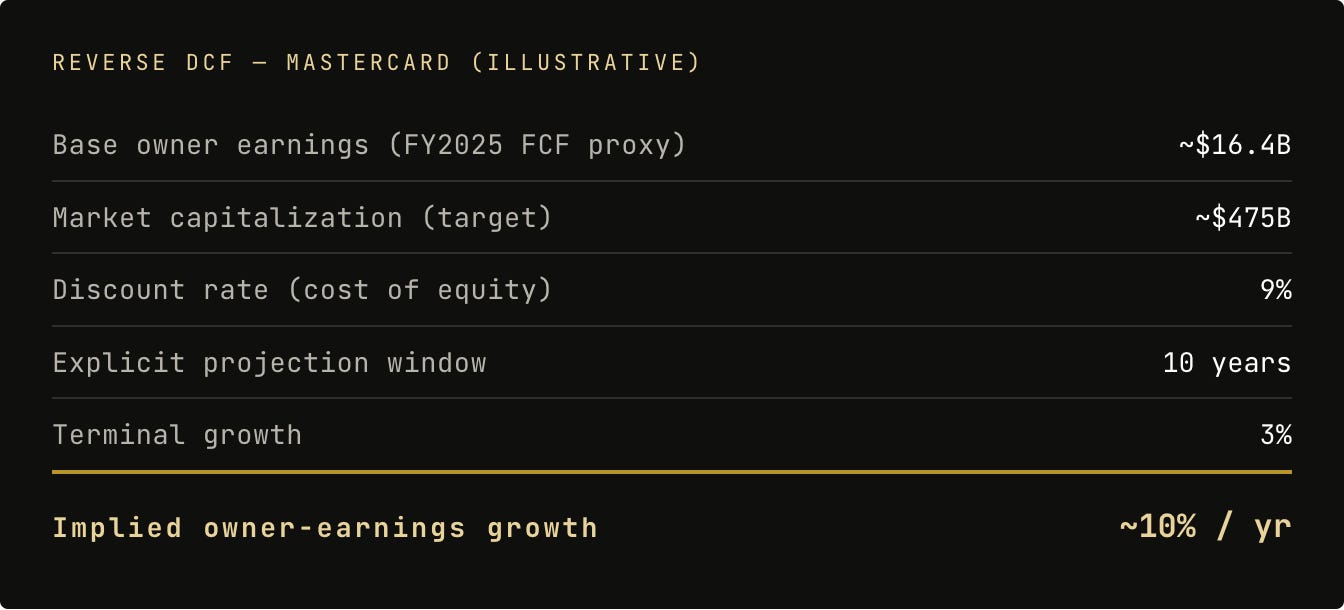
At the current price, the market is implying that Mastercard grows owner earnings at roughly 10% per year for a decade, then settles to 3% in perpetuity. That is the number the price is paying for. Notably, most of that value sits far out in time: in this model, only about a third of the $475 billion comes from the explicit ten-year cash flows, while the remaining two-thirds sits in the terminal value beyond year ten. A reverse DCF makes that duration explicit — a point that matters greatly in the interpretation.
Now hold that implied ~10% against reality. Mastercard has historically grown free cash flow at roughly 18-21% per year over the trailing three-, five-, and ten-year periods; revenue has compounded near 14% over five years, and earnings per share by roughly 17% over three years. Looking forward, analysts expect low-double-digit revenue growth in the near term, decelerating toward 10% over three years, with earnings per share growth around 15% in 2026 and 2027. Against that backdrop, the market’s implied ~10% owner-earnings growth for a decade sits below what the business has delivered historically and roughly in line with — or slightly below — the pace analysts expect over the medium term. The bar the price sets is, by the company’s own recent standards, undemanding.
Here is the crucial move, and the reason the reverse DCF matters. Whether that undemanding bar makes Mastercard “attractive” or “expensive” depends entirely on one question: can the business actually clear ~10% owner-earnings growth for a decade? If the durable trends — the global shift from cash to electronic payments, high-margin value-added services growing above 20%, cross-border volume, and new payment flows — keep the company compounding in the mid-teens, then a price paying for only ~10% is asking for less than the business can deliver, and the setup is favorable. If instead the overhangs weighing on the stock in 2026 — a roughly 14% drawdown year to date, U.S. interchange litigation and legislative risk, a U.K. regulatory probe into digital wallets, and fears that stablecoins disintermediate the networks — prove to be a permanent cap rather than transient noise, then ~10% may be exactly right, or even generous, and the price is not the bargain it first appears. The same business, at the same price, flips between attractive and expensive depending only on whether the implied growth rate is beatable — which is the entire point. The reverse DCF locates the expectation; it does not, by itself, tell the investor which way to bet.
Figures as of July 15, 2026. Price, share count, and market capitalization from public market data; FY2025 free cash flow (~$16.4B), operating cash flow (~$16.9B), and capex (~$489M) from reported fiscal-2025 results. Historical and forward growth figures are drawn from company filings and consensus analyst estimates. Free cash flow is used as a labeled proxy for owner earnings. Illustrative only — not a recommendation.
Section 5: The Interpretation
Reading the Implied Growth Rate — Where the Skill Lives
The mechanics of a reverse DCF are simple; the interpretation is where an investor adds value. Once the implied growth rate is known, it is compared against what the business can realistically achieve, and one of three conclusions follows.
Pricing in less than the business can deliver — Attractive
The implied growth rate sits below what the company has historically achieved and can plausibly sustain. The expectations bar is low and beatable. This is the setup a long-term investor wants — a good business the market has written off or is under-appreciating — because the margin for error is favorable, and even mediocre execution clears the bar.
Pricing in roughly what the business can deliver — Fair
The implied growth rate is in line with a reasonable forecast. The stock is fairly priced, and the investor’s return will approximate the growth the business actually produces — with little help from an expansion in expectations and little harm from a contraction. Recognizing this case is itself valuable: it says there is no edge here, and capital is better deployed elsewhere.
Pricing in more than the business can deliver — Avoid
The implied growth rate exceeds anything the company has sustained, or requires a trajectory that strains credulity — very high growth for a very long time. The stock is priced for perfection. Even excellent execution may not be enough, and any stumble triggers a painful re-rating. This is the setup to avoid, however wonderful the business, because the price already assumes the best case.
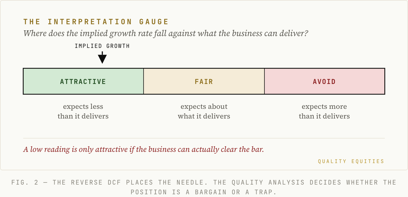
The judgment that makes all of this work is the assessment of whether the implied growth rate is achievable — and that judgment requires understanding the business: its moat, its reinvestment runway, its pricing power, and its historical growth. This is where every other Quality Equities framework feeds in. The reverse DCF tells the investor what the market expects; the quality analysis tells the investor whether that expectation is realistic. The ROIC piece, the moat framework, and the pricing power piece are the tools that answer the second question. The reverse DCF gives the market’s expectation; the moat, the ROIC, and the pricing power tell the investor whether it can be met.


There is one refinement that separates careful practitioners from casual ones: pay attention to how long the implied high growth must persist, not just how fast. The market’s expectation is often not an implausibly high growth rate for a few years, but a merely-high rate sustained for far longer than competition normally allows. A reverse DCF that requires 15% growth for fifteen years is frequently more demanding than one that requires 25% for three, precisely because durability is the rarer commodity. Recall that in the Mastercard example, two-thirds of the value sat in the years beyond the explicit decade. Durability of growth — the length of the runway — is where market expectations most often overreach, and where the quality analysis earns its keep.
Section 6: The Traps
The Ways a Reverse DCF Can Mislead
Most explanations of the reverse DCF teach the mechanic and stop. That omission is dangerous, because the tool misleads the careless user in specific, recurring ways. Four traps matter most.
Trap 1 — Peak or trough earnings as the base
A reverse DCF built on a cyclical business’s peak owner earnings will imply a modest growth rate and make the stock look cheap — precisely when it is most dangerous, because the base itself is about to fall. The same tool applied to trough earnings implies a heroic growth rate and makes a recovering business look expensive. For any cyclical business, the base must be normalized to mid-cycle owner earnings before the reverse DCF means anything at all. A low implied growth rate sitting on top of peak earnings is one of the most reliable traps in the entire discipline.
Trap 2 — Garbage owner earnings in
The reverse DCF inherits every flaw in the cash-flow figure it starts from. If the “owner earnings” base is really unadjusted GAAP net income, or a free cash flow number that quietly ignores stock-based compensation, or a figure inflated by one-time gains, then the implied growth rate is meaningless — a precise answer to a corrupted question. The discipline of the owner earnings calculation is a prerequisite for the reverse DCF, not an optional refinement to be applied later.
Trap 3 — Discount-rate sensitivity dressed up as insight
The implied growth rate moves with the discount rate the analyst chooses. In the Mastercard example, holding everything else constant, the implied growth rate ran from roughly 7% at an 8% discount rate, to about 10% at 9%, to roughly 12% at 10%. That is a wide band produced by nothing more than the choice of discount rate. An investor who wants a stock to look cheap can pick a low discount rate; one who wants it to look expensive can pick a high one — the same self-deception the forward DCF invites, smuggled in through a different door. The safeguard is to fix a consistent, defensible discount rate and apply it uniformly across every business analyzed, so that comparisons are genuinely apples to apples.
Trap 4 — Confusing a low implied growth rate with a good investment
A low implied growth rate means the market expects little — but sometimes the market is right to expect little, because the business is genuinely deteriorating. A reverse DCF showing that a stock is “pricing in almost no growth” is only bullish if the business can actually grow. On a company in structural decline, a low implied growth rate is not a bargain; it is an accurate forecast, and buying against it is walking into a value trap. The reverse DCF identifies low expectations; the quality analysis — the moat assessment above all — determines whether those expectations are too low or correctly low. This is the single most important discipline in using the tool.
The unifying lesson across all four is that the reverse DCF is only as good as the judgment surrounding it. Normalize the base, use a clean owner earnings figure, fix a consistent discount rate, and — above all — pair the implied growth rate with a real understanding of whether the business can beat it. The tool reveals the market’s expectation. It does not, by itself, tell the investor whether to bet with that expectation or against it.
Section 7: The Edge
What the Reverse DCF Gives You That Nothing Else Does
The reverse DCF is the single most useful valuation tool for a long-term investor because it aligns the analysis with the only thing that actually drives returns: the gap between what the market expects and what the business delivers. Three qualities set it apart.
First, it enforces intellectual honesty. A forward DCF lets an investor back into whatever answer they wanted by adjusting the growth rate until the model agrees. A reverse DCF takes the answer — the price — off the table and forces the investor to confront the market’s actual embedded expectation. It is far harder to fool oneself when the model hands over the market’s forecast and asks a single, uncomfortable question: can this business really do that? The discipline is in being made to answer.
Second, it reframes investing as a bet on expectations rather than on businesses. The reverse DCF makes explicit what the best investors understand intuitively — that returns come from the difference between reality and expectation, not from the quality of the business in isolation. Buying a great business at a price that already expects greatness earns nothing. Buying almost any business at a price that expects too little earns a great deal when it delivers merely something. The reverse DCF is the tool that locates those situations, because it shows precisely what the price is demanding.
Third, it is the bridge between quality analysis and price discipline. All the other frameworks — ROIC, owner earnings, moats, pricing power — describe how good a business is and how durably it can grow. The reverse DCF translates that quality assessment into an actual decision by testing it against what the market is charging. A wonderful business is a buy only when the reverse DCF shows the market is asking for less than the business can deliver. That test is the discipline that separates paying for quality from overpaying for it — the difference between a good business and a good investment.
Return on invested capital, owner earnings, moats, and pricing power establish how good a business is and how durably it can grow. The reverse DCF asks the final question: is the market already charging for all of that and more? It is the tool that turns quality analysis into an actual decision — and it is the method Quality Equities runs on every business it covers, stating explicitly what growth the current price assumes and whether the business can beat it.
Quality Equities publishes independent research for informational purposes only. Nothing published constitutes investment advice or a recommendation to buy or sell any security. The author may hold positions in securities discussed.
The value here is less in the model and more in the mindset. It forces the conversation away from “what do I think” to “what is already being assumed” - which is usually where the edge sits.